Friction Parameters
The model relies on the two-parameter Voellmy model widely used in Swiss snow engineering practice. To calibrate the RAMMS Voellmy-model, we used data from the SLF real scale avalanche test site in Vallée de la Sionne, VS, Switzerland. Special user features have been introduced into the model to account for variable surface roughness, vegetation and flow in forests. Swiss guideline suggestions for friction parameters (based on extensive model calibration) are also available for practical users.
Physical friction model
The model divides the frictional resistance into two parts: a dry-Coulomb type friction (coefficient $\mu$) that scales with the normal stress and a velocity-squared drag or viscous-turbulent friction (coefficient $\xi$). The frictional resistance $S$ (Pa) is then
where $\rho$ is the density, $g$ the gravitational acceleration, $\varphi$ the slope angle, $h$ the flow height and $u$ the vector $u=(u_x,u_y)^T$, consisting of the flow velocity in the x- and y-directions. The normal stress on the running surface, $\rho g h cos(\varphi)$, can be summarized in a single parameter $N$. The Voellmy model accounts for the resistance of the solid phase ($\mu$ is sometimes expressed as the tangent of the internal shear angle) and a viscous or turbulent fluid phase ($\xi$ was introduced by Voellmy by using hydrodynamic arguments). The friction coefficients are responsible for the behavior of the flow. $\mu$ dominates when the flow is close to stopping, $\xi$ dominates when the flow is running quickly.
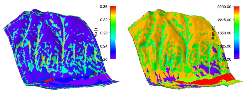
RAMMS::AVALANCHE offers a constant and a variable friction mode. If a calculation is done with constant friction values, of course, no terrain undulations and forest areas are considered. Therefore we suggest to use the variable friction values if possible. An automatic RAMMS procedure classifies friction values ($\mu$ and $\xi$) based on topographic data analysis (slope angle, altitude and curvature), forest information and global parameters return period and avalanche volume. $\mu$ and $\xi$ values are saved as ASCII files (called MuXi-files) and can be easily imported in GIS-Software (e.g. ArcGIS).
Automatic MuXi procedure
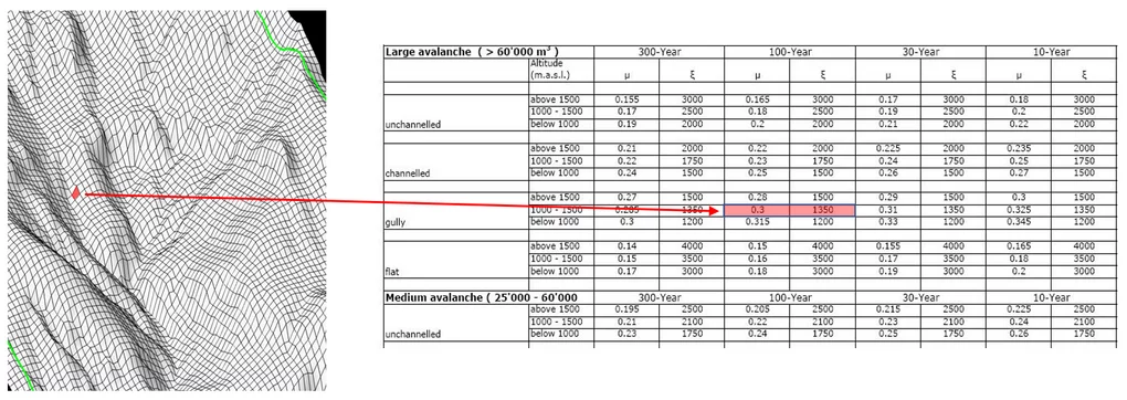
In the automatic procedure, $\mu$ and $\xi$ are calculated for every cell of the calculation based on the DEM. Slope angles and curvatures are calculated, whereas the altitude is known.
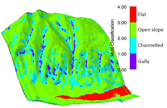
We use this information to automatically calculate the “track type” (flat, open slope, channeled, gully), see Figure below.
Together with the information about return period and avalanche volume (global parameters), $\mu$ and $\xi$ are derived from this table data.

Cohesion
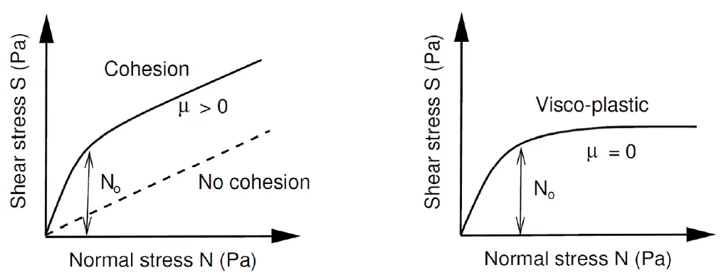
Since Version $1.6.20$ the basic Voellmy equation has been modified to include a cohesion. Many materials, like mud and snow, do not exhibit a simple linear relation ($\mu$ = constant), see Figure below. To model yield stress, we introduce the parameter $N_0$. With this approach it is possible to model ideal plastic materials. In this case $N_0$ serves as a yield stress and $\mu$ a “hardening” parameter. The new equation for the frictional resistance $S$ is then
$$S=\mu N + \frac{\rho g u^2}{\xi} + (1-\mu) N_0-(1-\mu)N_0 e^{-\frac{N}{N_0}}$$
where $N_0$ is the yield stress of the flowing material. Unlike a standard Mohr-Coulomb type relation this formula ensures that $S \rightarrow 0$ when both $N \rightarrow 0$ and $U \rightarrow 0$. It increases the shear stress and therefore causes the debris flow to stop earlier, depending on the value of $N_0$.
Curvature
Since Version 1.6.20, the normal force $N$ includes centrifugal forces arising from the terrain curvature. We use the method proposed by Fischer et al. (2012) which was specifically developed for RAMMS. The centrifugal acceleration $f$ is both a function of the flow velocity and terrain curvature. The acceleration is calculated according to
The matrix $K$ describes the track curvature in all directions, including the track “twist”. The centrifugal force is then
which is added to the normal force $N$. Typically this increases the friction, causing the flow to slow down in tortuous and twisted flow paths. It can change the location of the deposition once the flow leaves the gully. Curvature may be activated/deactivated in the Run Simulation window (tab Params) or via the menu ‘Help → Advanced… → Curvature’.
